1. Basic principles of transformer modeling

The actual modeling of isolated power transformers is more complicated. Not only the parasitic parameters between different windings, but also the windings and cores must be considered. parasitic capacitance between. In the high-frequency band, physical-level models can no longer meet the needs of high-frequency characteristics. The high-frequency broadband model needs to be freed from the constraints of physical modeling and modeled based on the FORSTER network principle.

2. Transformer physical level model

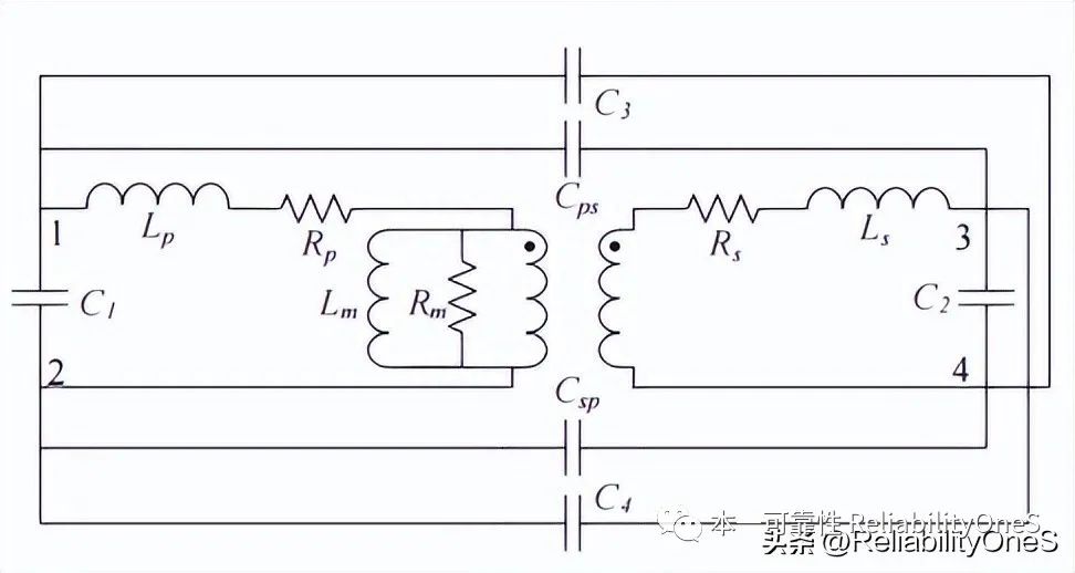
Figure 1 Transformer physical level model

3. High-frequency broadband modeling of isolation power transformer

3.1 Transformer excitation impedance model

Open both ends of the transformer and measure the impedance between terminals 1 and 2 of the primary side. The measured curve is shown in Figure 2.

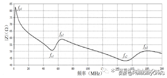
Figure 2 The measured impedance curve of the primary side when the transformer winding is open circuit

The impedance curve shows a multi-resonant distribution in the 200MHz frequency band. In order to facilitate the establishment and extraction of the excitation impedance model and parameters, the FOSTER network of RLC parallel units is used for modeling.

Modeling assumptions:

(1) The excitation impedance Zm is much larger than the primary and secondary leakage inductance impedances Zp and Zs. When calculating the Zm parameter, ignore the values of Zp and Zs. Influence;

(2) At 0Hz, Zm is resistive;

(3) At each peak resonance point It is parallel resonance at fpi, and it is determined by this unit, and has nothing to do with other units;

(4) It is series resonance at each valley resonance point fsi, and it is determined by this unit and Subsequently, the adjacent units are determined and have nothing to do with other units;

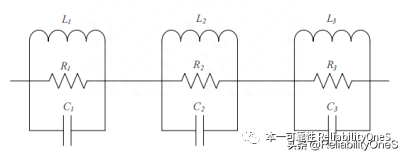
Figure 3 Three-level RLC parallel Zm network

Use a three-level RLC parallel unit to simulate the transformer excitation impedance Zm in the 200 MHz frequency range. Actual different transformers need to be analyzed based on the number of series and parallel resonance points in the actual impedance curve.

3.2 Transformer leakage impedance modeling

The modeling of transformer leakage impedance is also carried out through testing and fitting.

In the transformer leakage impedance modeling, it is assumed that Zm is much larger than Zp and Zs, that is, Zm is regarded as open circuit.

Short-circuit terminals 1, 3, and 4 and measure the input impedance at terminals 1 and 2 to obtain the transformer leakage impedance curve.

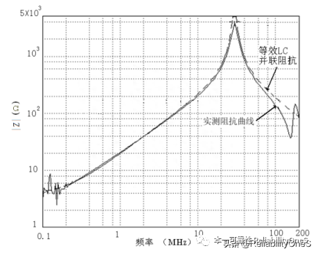
Figure 4 Zp input impedance curve

< p>(1) Considering the frequency variation effect of leakage inductance, series RL units and parallel RL units are used to better represent the primary/secondary leakage inductance;

< strong>(2) Distribute the measured leakage inductance value to the primary side leakage inductance and the secondary side leakage inductance in proportion to the square of the turns ratio;

(3) Primary/secondary side The resistance value of the winding is measured with an LCR meter, and the two sides of the transformer are represented by Rp, Lp1 to Rpi//Lpi and Rs, Ls1 to Rsi//Lsi.

3.3 Transformer primary and secondary capacitance model

The capacitance of the transformer primary and secondary windings is distributed in nature, and its broadband accurate model and Quantification is actually very difficult.

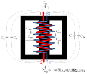
Figure 5 High-frequency equivalent parasitic parameter structure diagram< /p>

The transformer is fitted using six lumped capacitors. Among them, the primary winding capacitance C1 and the secondary winding capacitance C2 have been merged into Zm by their effects and are no longer extracted separately;

The capacitances C3, C4, Cps, and Csp between the primary and secondary windings are measured. and extracted by means of theoretical calculations. Due to the symmetry of the winding structure, C3=C4, Cps=Csp.

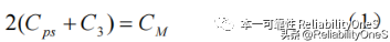
The specific extraction process and method of capacitance parameters are as follows: short-circuit the primary terminals 1 and 2 and the secondary terminals 3 and 4, use an impedance analyzer to measure the impedance of terminals 1 and 3, and obtain the impedance. Capacitance value CM, Figure 6 specifically shows the measured value in the 40MHz range. The measured relationship between capacitance CM, Cps, and C3 is consistent with Equation 1.

According to the research results, under the condition that the primary and secondary edges are uniform, Cps and C3 can be derived from the principle of electrostatic energy equivalence, which are approximately determined by equations 2 and 3. Among them, d is the gap between windings, w is the height of the winding, and C0 is the interlayer capacitance when the primary and secondary sides are equivalent to a flat thin plate.

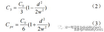
From the above three calculations, the winding can be extracted capacitance value.

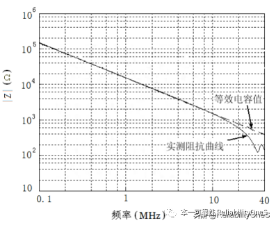
Figure 6 Capacitive impedance curve between the primary and secondary sides of the transformer

3.4 Transformer behavioral model and experimental verification

3.4.1 Behavioral model

The transformer excitation impedance model, leakage impedance model and capacitance model are combined to establish a behavioral model as shown in Figure 7.

Note: The aforementioned extraction of excitation impedance and leakage impedance ignores the interaction between them, so the extracted parameter value is only an initial value. In order to make the model more accurately approximate the measured impedance curve, some parameter values were fine-tuned based on the initial parameter values.

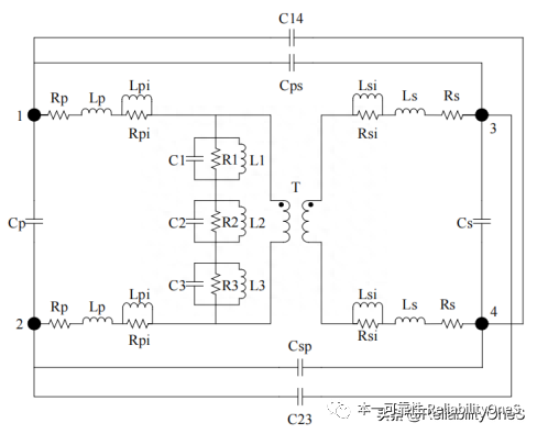
Figure 7 Transformer behavioral model

< p>3.4.2 Behavioral model wide-band impedance verification

Compare the wide-band impedance curves of simulation results and measured results.

Figures 8 to 10 show three sets of measured and simulated impedance curves of the transformer. The transformer behavior model can better fit the multi-resonance point frequency characteristics of the actual transformer within 200 MHz.

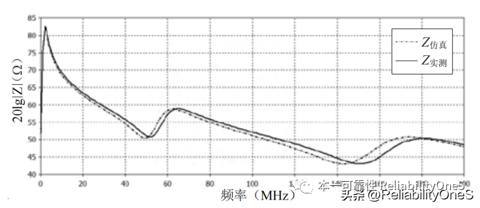
Figure 8-Testing terminals 1 and 2 with both ends open Input impedance curve

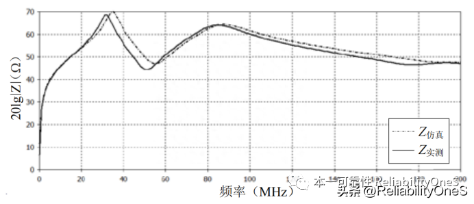
Figure 9 -3 and 4 terminals are short Connect and measure the input impedance curves of terminals 1 and 2

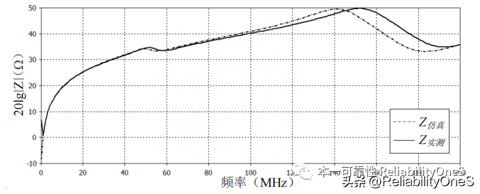
Figure 10 - Short-circuit terminals 1 and 2 to measure the input impedance curve of terminals 3 and 4

4. Thoughts and inspirations

(1) Traditional physics Level models are not suitable for high-frequency broadband modeling and need to be characterized with behavioral-level models;

(2) For complex distribution parameters, decoupling analysis needs to be performed first, and then Multi-dimensional coupling;

(3) Transformer broadband modeling uses the FORSTER network principle to better describe its impedance distribution curve and behavioral characteristics;

(4) The process of obtaining the distribution parameters of the transformer can be quickly obtained by combining testing and principle calculation analysis;